Introduction

A popular statistical calculation for variance is an unbiased estimator often called ‘sample variance’. In contrast, using the definition of variance is often called ‘population variance’ and it is a biased estimator. “The feeling that an unbiased estimator should be preferred to a biased estimator is prevalent in current statistical practice.” [1] Popular software, such as Excel, the Python statistics package and the R language, offer prominent functions named variance or var which default to calculating ‘sample variance’.

This document evaluates the use of this unbiased estimator with the simplest and most basic distribution: the Bernoulli distribution. The conclusion is the biased estimator called ‘population variance’ is a better point estimator than the unbiased ‘sample variance’, in the case of a Bernoulli distribution. It’s worth noting that ‘population variance’ is the Maximum Likelihood Estimator (MLE) for a Bernoulli distribution. This document will refer to ‘population variance’ as the MLE.

Useful applications of sample variance

This document focuses on point estimation of univariate Bernoulli distribution variance. Although similar conclusions can be drawn for a univariate normal distribution, these results do not generalize to multivariate distributions [2].

Point estimation is not the only application for sample variance. Sample variance will precisely generate a Chi-square distribution given normally distributed samples of unit variance [1]. The Chi-square distribution in turn is part of the t-distribution which is the basis of the popular t-test. Although sample variance can be point estimator, it can be very useful as a function that is not a point estimator.

A bias against bias

A binary categorization of estimators, such as ‘biased’ vs ‘unbiased’, benefits from simplicity, understandability and ease of communication. “The very terminology of the theory of unbiased estimation seems to make the use of unbiased estimators highly desirable.” [1] Clearly ‘biased’ does not sound good. But is this property of an estimator, independent of its negative label, actually undesirable.

We consider a parable that is analogous to choosing estimators.

A ‘biased’ bus

Imagine a commuter debating between two buses. Both buses will pass the commuter’s destination after 40 blocks.

Bus A)

Unfortunately, the driver of bus A is unreliable and easily distracted. Bus A stops one block short (39 blocks) 90% of the time and 9 blocks too far (49 blocks) 10% of the time. The expected (average) travel distance on Bus A is 40 blocks.

Bus B)

Bus B always stops after 39 blocks.

Applying terms from statistics, bus B is the ‘biased’ bus because it systematically stops one block too soon. Bus A on the other hand is the ‘unbiased’ bus because the expected travel distance is 40 blocks.

Which bus should the commuter take? The commuter could follow the rule that ‘unbiased’ buses are preferable to ‘biased’ buses.

Better measures of desirability

The fundamental problem with choosing the ‘unbiased’ bus A is that the too-short and too-long distances cancel each other out. A more rational approach would evaluate the average utility of the various distances, not the average distance. The most popular approach is to evaluate loss of utility with a loss function. In the bus parable, this loss function could be the distance the commuter will need to walk after getting off the bus. This measure is called Mean Absolute Error (MAE).

A more common choice with extremely convenient mathematical properties is Mean Squared Error (MSE). A well known decomposition of MSE is the sum of the estimator variance plus the square of the bias. Although bias by itself may not be a good measure of quality, the magnitude of bias might be the important component of MSE depending on the relative magnitudes of estimator variance vs bias.

Bernoulli distribution

We now switch to an actual mathematical example rather than an illustrative parable. Consider data generated by a Bernoulli distribution with probability $p$. The variance of this data generating process is $p (1-p)$.

The Maximum Likelihood Estimator (often called ‘population variance’) is $$M = \frac{1}{n} \sum_{j=1}^n \left( X_i - \frac{1}{n} \sum_{j=1}^n X_j \right)^2$$ where $X_i$ are independent samples of data generated from the distribution.

A well established result for any $p$ is the expected value of the MLE $${\operatorname{E}\!\left[{ M}\right]} = \frac{n-1}{n} p (1-p)$$

By multiplying the MLE by $\frac{n}{n-1}$ we get what is often called the ‘sample variance’ and it is an unbiased estimator.

We now perform simulations to compare the performance of these two estimators.

Simulation code is in a Jupyter notebook “biased_estimator” : [as HTML] [as .ipynb file]

Estimating when $p = 0.5$

Consider the distribution of simulated estimates for n = 32 and $p = 0.5$:

The true variance to be estimated is $$p (1-p) = 0.5 \cdot (1-0.5) = 0.25$$

The sample variance is as follows:

At first glance it might seem the unbiased estimator is preferable. But consider that the range of possible estimands is $[0, 0.25]$. Even before observing one single data point, we know that the variance to be estimated can not be greater than $0.25$.

In fact, in the specific case of $p = 0.5$ we should fully expect all estimates to be equal or less than the estimand and none greater than.

A third estimator can be created by taking the minimum of $0.25$ and the unbiased estimator. But this will no longer be an unbiased estimator. It is clearly better at estimating $p$ than the unbiased estimator. But is this new biased estimator better than the biased MLE?

For distributions with $p$ near $0.5$ the unbiased estimator makes an irrational trade off of choosing impossible values of variance so that the error on average is zero. It is a similar trade-off of choosing the ‘unbiased’ bus over the ‘biased’ bus so that the distance traveled is on average the desired distance.

Probability of Impossible Estimand

Another possible loss function assigns $1$ to an estimate if it is an impossible estimand and $0$ otherwise. This document will refer to the expectation of this loss function as the ‘Probability of Impossible Estimand’ (PIE).

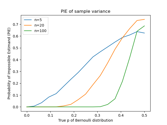
We now consider PIE across all possible values of $p$. For the biased MLE, PIE is always zero. For the unbiased sample variance it depends on $p$ and the number of samples $n$. Here are simulations that summarize the trend:

We see high PIE for all distributions with $p$ near $0.5$. For lower numbers of samples $n$, notable PIE values expand into most of the range of possible distributions.

These issues with PIE are specific to distributions with bounded variance and not distributions with unbounded variance (e.g. the normal distribution).

Overall performance across all $p$

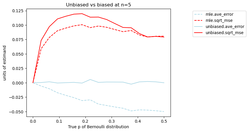
We finish looking at the performance in both PIE and MSE of both estimators. First we look at MSE and average error (bias) for both sample variance and the MLE for $n=5$:

We see that MSE is generally smaller with the MLE than sample variance for small sample sizes. So although the sample variance maintains an average error around zero, it does so at the cost of worse overall performance, as evaluated by MSE.

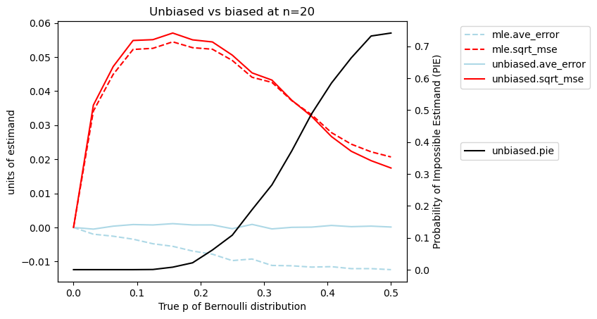
For a sample size of $n=20$ the line of PIE is added as a black line:

Here we see again that for low values of $p$ the MLE has better MSE than sample variance. For higher values of $p$, sample variance does achieve improved MSE but it does so at the cost of significantly increased PIE.

Conclusion

When evaluated as a point estimator for a Bernoulli distribution, the sample variance is not more desirable than the MLE. In fact, when evaluated in the context of two loss functions, MSE and PIE, the MLE is actually more desirable despite its label of being ‘biased’.

Acknowledgements

Thanks to Peter Ralph for some points on statistics in this document.

References